Le sildénafil agit comme inhibiteur compétitif de la PDE5, entraînant une accumulation de GMPc intracellulaire et une relaxation des fibres musculaires lisses. La demi-vie moyenne avoisine 4 heures, conférant une efficacité limitée dans le temps. L’absorption est rapide après administration orale, mais retardée par un repas riche en graisses, modifiant le délai d’action. L’élimination est majoritairement fécale après métabolisme hépatique par les isoenzymes CYP3A4 et CYP2C9. Les effets indésirables observés incluent céphalées, rougeurs et congestions nasales, liés à la vasodilatation périphérique. Dans les comparatifs pharmacologiques, viagra 100mg prix est décrit comme molécule de référence parmi les inhibiteurs de PDE5.
Xisgapeio.udc.es
XI Congreso Galego de Estat´ıstica e Investigaci´
Dependent Functional Regression Models for detecting influenza epidemics
Manuel Oviedo de la Fuente1, Manuel Febrero-Bande1 and M. Pilar Mu˜
1Department of Statistics and Operations Research, Universidade de Santiago de Compostela2Department of Statistics and Operations Research, Universitat Politcnica de Catalunya
The objective of this work is to estimate the space-time components of a contagiousdisease, such as the flu, using functional linear models (FLM). We study the conditionsfor the fit of the parameters of FLM by analyzing spatial dependence (each curve isindexed in a grid), or temporal dependence (each curve is indexed in time) and evaluatethe forecasting performance.
keywords: Linear Models, influenza, count data, basis representation, epidemiological surveil-
lance, least squares, functional dependent data.
Surveillance systems must critically have precise indicators that detect in advance various epi-
demics that may occur. One of the problems that concern epidemiologists the most on a globallevel is the outbreak of flu, both for sick leave caused by this illness as well as the number of deaths. In addition, this disease is highly contagious. To have accurate estimates of the incidence of flu isvitally important both for public health services and citizens in general. This information shouldallow patients to be informed of possible contagions in advance while also reducing the spred ofpossible contagions. Controlling this contagion is very important because influenza causes moremorbidity than any other vaccine-preventable illness Monto et al. (2002).
The statistical methodology for forecasting incidences of influenza in particular and contagious
diseases in general has changed over time. One of the first works on time series was that proposed byChoi and Tacker (1981), where they fit an ARIMA model for estimating pneumonia and influenzamortality in order to know the number of deaths caused by these diseases. Recently, Dushoff etal. (2006) investigated how cold temperatures contribute to excess seasonal mortality through aregression model and Mu˜
noz et al. (2011) studied the relationships between influenza morbidity
and all causes of mortality, taking into account influenza vaccination coverage.
In order to monitor infectious diseases, an alternative to these procedures is that proposed by
Hohle and Paul (2008), which consists of applying count data charts to monitor these kinds of timeseries. An approach that could also be applied to infectious diseases is to take into account thegeographical component in statistical models in addition to the temporal evolution, i.e., how farapart or close together the detected cases are. The number of contributions to this methodology isgrowing steadily through disease mapping. As examples, we can cite the recent papers of Ugarteet al (2010) and Paul and Held (2011). The common denominator to all of them is that theyapply different statistical methodologies to multivariate time series (hierarchical Bayesian space-time, mixed models, P–splines, conditional autoregressive (CAR), and a long etcetera) of infectiousdisease counts, collected in different geographic areas.
Functional data analysis (FDA) is a very active area of research in recent years. As a start-
ing point, we discuss the functional linear models (FLM) treated in the literature by Ramsayand Silverman, (2005). In recent years, several methods have been proposed for analyzing high-dimensional data; some of them fall under the category of functional data analysis, and only afew of them believe this functional data presents either spatial Delicado et al (2010) or temporalDamon and Guillas (2005) dependencies. This work introduces a functional model which includesthe two components, spatial and temporal.
The objective of this work is to estimate the space-time components of a contagious disease,
such as the flu, using functional regression models and to predict the rate of incidence of thisdisease out of sample for horizons of one week to a quarter of a year. In particularity, we are inter
2. Methodology: Functional Regression Models
Regression models are those techniques for modeling and analyzing the relationship between
a dependent variable and one or more independent variables. When one of the variables havea functional nature, we have functional regression models.
functional regression models where the response variable y is scalar and at least, there is onefunctional covariate X(t).
Let X(t) be a functional r.v. taking values in H = L2[0, T ]. In the functional linear model
(FLM), the scalar response y is modeled as a linear function of covariate X(t) as follows,
where ·, · denotes the inner product on L2 and
is the error term with covariance matrix Σ. The
estimation of the functional parameter β is done by minimizing the RSS:
Different methods have been proposed to search for the ˆ
The general form of Σ is given by a function of unknown parameter θ, Σ = σ2Σ(θ). If Σ
is known, the best linear unbiased estimator (BLUE) of functional parameter β(t) is given by afunctional version of the generalized least squares estimator (GLSE) of β
X is the representation of functional data X(t) in a basis expansion. Note that, if
Σ = I, the model includes the classical functional linear regression models (FLM) which entailsindependent errors structure, i.e., the GLSE in equation 2 reduces to the ordinary least squaresestimator (OLSE).
An extension of the FLM model for dependent data require to study the structure of Σ: an-
alyzing temporal dependence (each curve is indexed in time), spatial dependence (each curve isindexed in a grid) or both.
Serial correlation structuresIn temporal dependences typically assumes that errors are observed at integer time points. A
common method of modeling serial correlation structures is to estimate an autoregressive movingaverage model ARMA of the errors.
t = φ t−1 + . . . + φq t−p + as + θat−1 + . . . + θq at−q
where at are a independent and centered errors, E [at] = 0, V ar [at] = σ2.
In this case, the covariance matrix of the errors Σ = σ2diag (Σ(Φ)) depends of the p + q param-
eters Φ = {φ1, . . . , φp, θ1, . . . , θq}. For example, we can model serial correlation using the simplestand useful AR(1) model. Its covariance matrix is Σ = σ2Σ(φ) where Σi,j = φ|i−j|.
Spatial Correlation StructuresThis structure appear when the data are measured at spatial location vector, to simplify the
data are in a 2-dimensional vector (x, y). There estimation of spatial correlation structures isbased on shape of semivariogram models as Exponential, Spherical, Linear, among others, seeCressie, (1993). For example, the exponential semivariogram γ(·) without nugget effect is given
by γ(σ2, ρ) = σ2 1 − es/ρ where σ2 is the sill, ρ is the range (correlation parameter) and s thedistance si,j = dist ((xi, yi) − (xj, yj)). The semivariogram is related the covariance matrix of theerrors as γ (·) = σ2I − Σ so in this case we need know σ2, ρ to compose Σ = σ2es/ρ.
Group covariance structuresThe correlation structures are used to model dependence among the within-group errors. Now,
observations in different groups are assumed independent, so Σ is a block diagonal matrix of thecorrelation matrices per group, Σ = σ2diag (Σ1(Φ), . . . , Σk(Φ)).
Heterogeneous group covariance structuresThis structure gives rise to independent observations, however with different variability accord-
ing group level since different levels are mutually independent. The heteroscedastic model requireknow different variances for each level of the grouping variable. The covariance matrix of errorsis Σ = diag σ2Σ
is the variance of the group level i. We can also
model different dependence parameter by group level Σ = diag σ2Σ
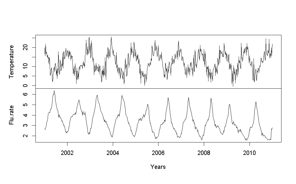
We analyze the weekly influenza reported at s = 53 regions during the period 2001 − 2011 in
Galicia. The data has been obtained from the Galician Influenza Surveillance Program. For eachregion, temperatures (downloaded from http://www.meteogalicia.es/) and incidence rate of flu ofprevious days and weeks respectively are used as covariates, see Figure 1.
Figure 1: Weekly average temperature (up) and influenza rate (down) on the Galician regions.
influenza rate for epidemic period and non–epidemic period.
We apply the functional dynamic models for detecting the outbreak of influenza, where the
functional regression model is required to use influenza circulation data at observed time t inregion s. We use the first n times to fit the model. The proposed model estimates the incidencein the region s and time n + 5, Raten+5,s. The explanatory variables to introduce in the modelsare: the incidence of previous weeks Raten,s(t) = (Raten−13,s, . . . , Raten,s), the temperature andit first derivative of the previous 14 days T emp(s), T emp.d1(s) respectively. Figure 3 shows theestimation of the functional parameter β for each covariate. All functional covariate effects aresignificant. The incidence rate is increased by reason of the last values of ˆ
last 3 weeks). When the temperature decreases the incidence rate increases.
The next 52 times has been used to check the predictions for model which assumes independent
errors and autoregressive errors AR(1) respectively, see table 1. Akaike information criterion (AIC),
Figure 2: In left, influenza rate for epidemic period (weeks 40 − 20) and in right, non–epidemicperiod (weeks 21 − 39).
Ratet+5,s ∼ Raten,s(t) + T emp(s) + T emp.d1(s)
Ratet+5,s ∼ Raten,s(t) + T emp(s) + T emp.d1(s) φ = 0.77
Table 1: Predictions errors for functional regression models.
mean square error of prediction (MSE) and mean relative error of prediction (MRE) have beencomputed for each model.
We propose a flexible and generic procedure to model influenza using functional models. This workconsiders the extension of functional linear models with independent errors to dependent errors. We study how to incorporate the temporal and spatial dependence structures into functional modeland we evaluate the forecasting performance. Furthermore, the results might be more precise, ifwe introduce other epidemiological data such as data of influenza virus type, vaccination status,age or gender of infected, for example.
This work was supported by grants MTM2008-03010 from the Ministerio de Ciencia e Innovaci´
10MDS207015PR from the Xunta de Galicia and GI-1914 MODESTYA-Modelos de optimizaci´
Efron, B. and Tibshirani, R. (1994) An introduction to the Bootstrap. Chapman & Hall.
Monto, A, Pichichero, M. Blanckenberg, S. et al.
Zanamivir Prophylaxis: An Effective Strategy
for the Prevention of Influenza Types A and B within Households. J Infect Dis. (2002) 186(11),1582–1588.
Choi, K. adn Thacker, S. (1981) An evaluation of influenza mortality surveillance, 1962–1979. AmJ Epidemiol 113, 215–26.
Dushoff, J., Plotkin, J.B., Viboud, C, Earn, D. and Simonsen, L. (2006). Mortality due to Influenzain the United States, An Annualized Regression Approach Using Multiple Cause Mortality Data. Am J Epidemiol, 163, 181-187.
noz, M.P., Soldevila, N., Martnez, A., Carmona, G., Batalla, J., Acosta, L. and Domnguez,
A. (2011) Influenza vaccine coverage, influenza-associated morbidity and all-cause mortality inCatalonia (Spain). Vaccine 29, 5047–5052.
Hohle, M. and Paul, M. (2008) Count data regression charts for the monitoring of surveillancetime series. Computational Statistics and Data Analysis 52, 4357-68.
Ugarte, M.D., Goicoa, T. and Militino, A.F. (2010) Spatio-temporal modeling of mortality risksusing penalized splines. Environmetrics, 21, 270–289.
Paul, M. and Held, L. Predictive assessment of a non-linear random effects model for multivariatetime series of infectious disease counts. Statistics in Medicine (2011), 30, 1118–1136.
Delicado,P. ,Giraldo, R., Comas C. and Mateu J. (2010). Statistics for spatial functional data:some recent contributions. Environmetrics 21, 224–239.
Damon, J. and Guillas, S. (2005) Estimation and Simulation of Autoregressive Hilbertian Processeswith Exogenous Variables. Statistical Inference for Stochastic Processes 8, 185-204.
Febrero Bande, M. and Oviedo de la Fuente, M. (2012). Statistical Computing in Functional DataAnalysis: The R Package fda.usc, Journal of Statistical Software,51(4), 1–28,http://www.jstatsoft.org/v51/i04/.
Volumes agents classés par le Monographies du CIRC, 1-100N ° CAS Année Volume Agent groupe000075-07-0 Acétaldéhyde associés à la consommation de boissons alcooliséesboissons 1 100E en préparationvapeurs acides, minéral fort 1 54, 100F en préparation001402-68-2 aflatoxines 1 56, 82, 100F en préparationBoissons alcoolisées 1 44, 96, 100E en préparationLa production d'aluminium 1 34, Su
 by γ(σ2, ρ) = σ2 1 − es/ρ where σ2 is the sill, ρ is the range (correlation parameter) and s thedistance si,j = dist ((xi, yi) − (xj, yj)). The semivariogram is related the covariance matrix of theerrors as γ (·) = σ2I − Σ so in this case we need know σ2, ρ to compose Σ = σ2es/ρ.
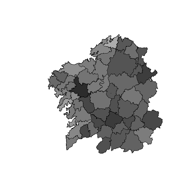
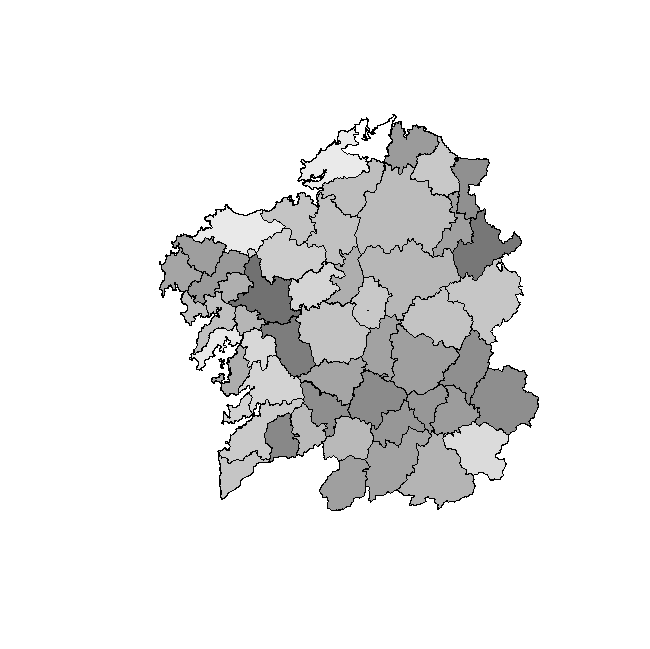 Figure 2: In left, influenza rate for epidemic period (weeks 40 − 20) and in right, non–epidemicperiod (weeks 21 − 39).